 |
|
|
Computational FinanceThis version of the paper is for reading online and will not give good results when printed. Please download either the Postscript or PDF version for printing a hardcopy. If you cannot see the equations online please read these notes. International Journal of Neural Systems, Vol. 8,
No.5 (October, 1997). A First Application of Independent Component Analysis to Extracting Structure from Stock Returns Andrew D. Back back@brain.riken.go.jp Andreas S. Weigend aweigend@stern.nyu.edu
In this paper we consider the application of a signal processing technique known as independent component analysis (ICA) or blind source separation, to multivariate financial time series such as a portfolio of stocks. The key idea of ICA is to linearly map the observed multivariate time series into a new space of statistically independent components (ICs). We apply ICA to three years of daily returns of the 28 largest Japanese stocks and compare the results with those obtained using principal component analysis (PCA). The results indicate that the estimated ICs fall into two categories, (i) infrequent but large shocks (responsible for the major changes in the stock prices), and (ii) frequent smaller fluctuations (contributing little to the overall level of the stocks). We show that the overall stock price can be reconstructed surprisingly well by using a small number of thresholded weighted ICs. In contrast, when using shocks derived from principal components instead of independent components, the reconstructed price is less similar to the original one. Independent component analysis is shown to be a potentially powerful method of analysing and understanding driving mechanisms in financial time series. 1 IntroductionWhat drives the movements of a financial time series? This surely is a question of interest to many, ranging from researchers who wish to understand financial markets, to traders who will benefit from such knowledge. Can modern knowledge discovery and data mining techniques help discover some of the underlying forces? In this paper, we focus on a new technique which to our knowledge has not been used in any significant application to financial or econometric problems1. The method is known as independent component analysis (ICA) and is also referred to as blind source separation [29,32,22]. The central assumption is that an observed multivariate time series (such as daily stock returns) reflect the reaction of a system (such as the stock market) to a few statistically independent time series. ICA seeks to extract out these independent components (ICs) as well as the mixing process. ICA can be expressed in terms of the related concepts of entropy [6], mutual information [3], contrast functions [22] and other measures of the statistical independence of signals. For independent signals, the joint probability can be factorized into the product of the marginal probabilities. Therefore the independent components can be found by minimizing the Kullback-Leibler divergence between the joint probability and marginal probabilities of the output signals [3]. Hence, the goal of finding statistically independent components can be expressed in several ways:
From this basis, algorithms can be derived to extract the desired independent components. In general, these algorithms can be considered as unsupervised learning procedures. Recent reviews are given in [2,12,51,52]. Independent component analysis can also be contrasted with principal component analysis (PCA) and so we give a brief comparison of the two methods here. Both ICA and PCA linearly transform the observed signals into components. The key difference however, is in the type of components obtained. The goal of PCA is to obtain principal components which are uncorrelated. Moreover, PCA gives projections of the data in the direction of the maximum variance. The principal components (PCs) are ordered in terms of their variances: the first PC defines the direction that captures the maximum variance possible, the second PC defines (in the remaining orthogonal subspace) the direction of maximum variance, and so forth. In ICA however, we seek to obtain statistically independent components. PCA algorithms use only second order statistical information. On the other hand, ICA algorithms may use higher order2 statistical information for separating the signals, see for example [11,22]. For this reason non-Gaussian signals (or at most, one Gaussian signal) are normally required for ICA algorithms based on higher order statistics. For PCA algorithms however, the higher order statistical information provided by such non-Gaussian signals is not required or used, hence the signals in this case can be Gaussian. PCA algorithms can be implemented with batch algorithms or with on-line algorithms. Examples of on-line or ``neural'' PCA algorithms include [9,4,45]. This paper is organized in the following way. Section 2 provides a background to ICA and a guide to some of the algorithms available. Section 3 discusses some issues concerning the general application of ICA to financial time series. Our specific experimental results for the application of ICA to Japanese equity data are given in section 4. In this section we compare results obtained using both ICA and PCA. Section 5 draws some conclusions about the use of ICA in financial time series. 2 ICA in General2.1 Independent Component AnalysisICA denotes the process of taking a set of measured signal vectors, x, and extracting from them a (new) set of statistically independent vectors, y, called the independent components or the sources. They are estimates of the original source signals which are assumed to have been mixed in some prescribed manner to form the observed signals.
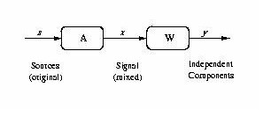
Figure 1 shows the most basic form of ICA. We use the following notation: We observe a multivariate time series { xi(t)} , i = 1,...,n, consisting of n values at each time step t. We assume that it is the result of a mixing process
Using the instantaneous observation vector x(t) = [x1(t),x2(t),...,xn(t)]˘ where ˘ indicates the transpose operator, the problem is to find a demixing matrix W such that
where A is the unknown mixing matrix. We assume throughout this paper that there are as many observed signals as there are sources, hence A is a square n ×n matrix. If W = A-1, then y(t) = s(t), and perfect separation occurs. In general, it is only possible to find W such that WA = PD where P is a permutation matrix and D is a diagonal scaling matrix [55]. To find such a matrix W, the following assumptions are made:
In this paper, we only consider the case when the mixtures occur instantaneously in time. It is also of interest to consider models based on multichannel blind deconvolution [33,59,44,57,64,47] however we do not do this here. 2.2 Algorithms for ICAThe earliest ICA algorithm that we are aware of and one which generated much interest in the field is that proposed by [29]. Since then, various approaches have been proposed in the literature to implement ICA. These include: minimizing higher order moments [11] or higher order cumulants3 [14], minimization of mutual information of the outputs or maximization of the output entropy [6], minimization of the Kullback-Leibler divergence between the joint and the product of the marginal distributions of the outputs [3]. ICA algorithms are typically implemented in either off-line (batch) form or using an on-line approach. A standard approach for batch ICA algorithms is the following two-stage procedure [8,14].
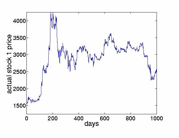
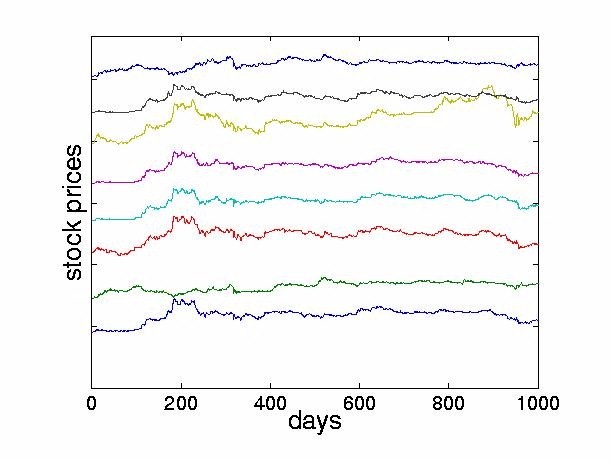
This approach is sometimes referred to as ``decorrelation and rotation''. Note that this approach relies on the measured signals being non-Gaussian. For Gaussian signals, the higher order statistics are zero already and so no meaningful separation can be achieved by ICA methods. For non-Gaussian random signals the implication is that not only should the signals be uncorrelated, but that the higher order cross-statistics (eg. moments or cumulants) are zeroed. The empirical study carried out in this paper uses the JADE (Joint Approximate Diagonalization of Eigenmatrices) algorithm [14] which is a batch algorithm and is an efficient version of the above two step procedure. The first stage is performed by computing the sample covariance matrix, giving the second order statistics of the observed outputs. From this, a matrix is computed by eigendecomposition which whitens the observed data. The second stage consists of finding a rotation matrix which jointly diagonalizes eigenmatrices formed from the fourth order cumulants of the whitened data. The outputs from this stage are the independent components. For specific details of the algorithm, the reader is referred to [14]. The JADE algorithm has been extended by [50]. Other examples of two-step methods were proposed in [11,21,8]. A wide variety of on-line algorithms have been proposed [3,6,15-23,27,28,31,34-39,43,46,49]. Many of these algorithms are sometimes referred to as ``neural" learning algorithms. They employ a cost function which is optimized by adjusting the demixing matrix to increase independence of outputs. ICA algorithms have been developed recently using the natural gradient approach [3,1]. A similar approach was independently derived by Cardoso [13] who referred to it as a relative gradient algorithm. This theoretically sound modification to the usual on-line updating algorithm overcomes the problem of having to perform matrix inversions at each time step and therefore permits significantly faster convergence. Another approach, known as contextual ICA was developed in [48]. In this method, which is based on maximum likelihood estimation, the source distributions are modeled and the temporal nature of the signals is used to derive the demixing matrix. The density functions of the input sources are estimated using past values of the outputs. This algorithm proved to be effective in separating signals having colored Gaussian distributions or low kurtosis. The ICA framework has also been extended to allow for nonlinear mixing. One of the first approaches in this area was given in [10]. More recently, an information theoretic approach to estimating sources assumed to be mixed and passed through an invertible nonlinear function was proposed in [63] and [62]. Unsupervised learning algorithms based on maximizing entropy and minimizing mutual information are described in [61]. Lin, Grier and Cowan describe a local version of ICA [38]. Rather than finding one global coordinate transformation, local ICAs are carried out for subsets of the data. While using invertible transformations, this is a promising way to express global nonlinearities. ICA algorithms for mixed and convolved signals have also been considered, see for example [24,33,44,47,52,57,59,64]. 3 ICA in Finance3.1 Reasons to Explore ICA in FinanceICA provides a mechanism of decomposing a given signal into statistically independent components. The goal of this paper is to explore whether ICA can give some indication of the underlying structure of the stock market. The hope is to find interpretable factors of instantaneous stock returns. Such factors could include news (government intervention, natural or man-made disasters, political upheaval), response to very large trades and of course, unexplained noise. Ultimately, we hope that this might yield new ways of analyzing and forecasting financial time series, contributing to a better understanding of financial markets. 3.2 PreprocessingLike most time series approaches, ICA requires the observed signals to be stationary4. In this paper, we transform the nonstationary stock prices p(t), to stock returns by taking the difference between successive values of the prices, x(t) = p(t)-p(t-1). Given the relatively large change in price levels over the few years of data, an alternative would have been to use relative returns, log(p(t)) - log(p(t-1)), describing geometric growth as opposed to additive growth. 4 Analyzing Stock Returns with ICA4.1 Description of the DataTo investigate the effectiveness of ICA techniques for financial time series, we apply ICA to data from the Tokyo Stock Exchange. We use daily closing prices from 1986 until 19895 of the 28 largest firms, listed in the Appendix. Figure 2 shows the stock price of the first company in our set, the Bank of Tokyo-Mitsubishi, between August 1986 and July 1988. For the same time interval, Figure 3 displays the movements of the eight largest stocks, offset from each other for clarity.
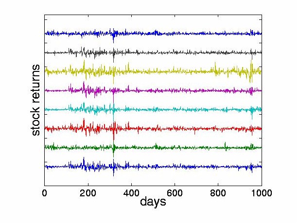
The preprocessing consists of three steps: we obtain the daily stock returns as indicated in Section 3.2, subtract the mean of each stock, and normalize the resulting values to lie within the range [ -1,1] . Figure 4 shows these normalized stock returns.
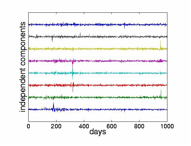
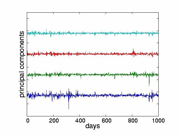
4.2 Structure of the Independent ComponentsWe performed ICA on the stock returns using the JADE algorithm [14] described in Section 2.2. In all the experiments, we assume that the number of stocks equals the number of sources supplied to the mixing model. In the results presented here, all 28 stocks are used as inputs in the ICA. However for clarity, the figures only display the first few ICs6. Figure 5 shows a subset of eight ICs obtained from the algorithm. Note that the goal of statistical independence forces the 1987 crash to be carried by only a few components.
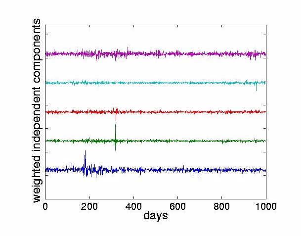
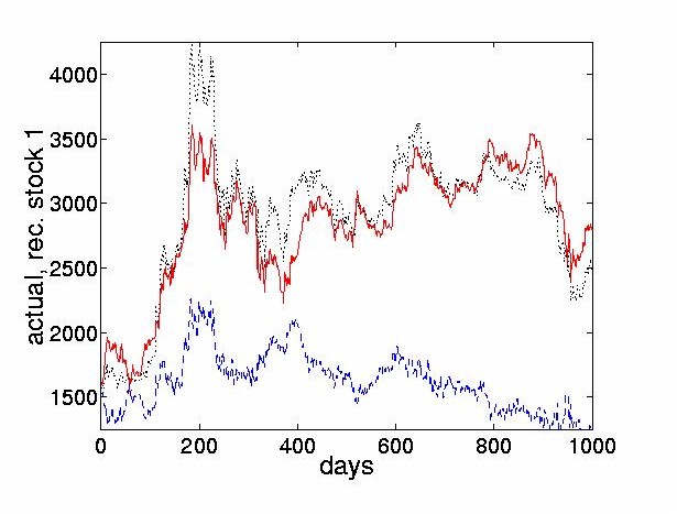
We now present the analysis of a specific stock, the Bank of Tokyo-Mitsubishi. The contributions of the ICs to any given stock can be found as follows. For a given stock return, there is a corresponding row of the mixing matrix A used to weight the independent components. By multiplying the corresponding row of A with the ICs, we obtain the weighted ICs. We define dominant ICs to be those ICs with the largest maximum signal amplitudes. They have the largest effect on the reconstructed stock price. In contrast, other criteria, such as the variance, would focus not on the largest value but on the average. Figure 6 weights the ICs with the the first row of the mixing matrix which corresponds to the Bank of Tokyo-Mitsubishi. The four traces at the bottom show the four most dominant ICs for this stock. From the usual mixing process given by Eq. (1), we can obtain the reconstruction of the ith stock return in terms of the estimated ICs as
where yk(t-j) is the value of the kth estimated IC at time t-j and aik is the weight in the ith row, kth column of the estimated mixing matrix A (obtained as the inverse of the demixing matrix W). We define the weighted ICs for the ith observed signal (stock return) as
In this paper, we rank the weighted ICs with respect to the first stock return. Therefore, we multiply the ICs with the first row of the mixing matrix and use a1k k = 1,..,n to obtain the weighted ICs. The weighted ICs are then sorted7 using an LĄ norm since we are most interested in showing just those ICs which cause the maximum price change in a particular stock.
The ICs obtained from the stock returns reveal the following aspects:
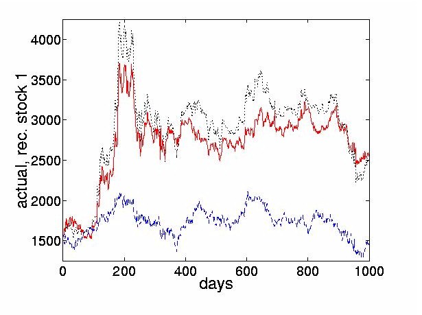
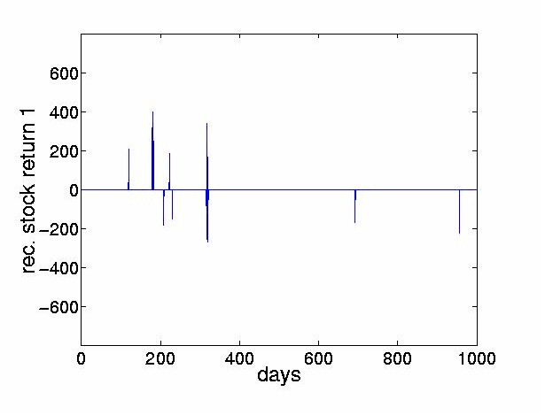
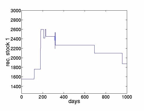
Figure 7 shows the reconstructed price obtained using the four most dominant weighted ICs and compares it to the sum of the remaining 24 nondominant weighted ICs. 4.3 Thresholded ICs Characterize Turning PointsThe preceding section discussed the effect of a lossy reconstruction of the original prices, obtained by considering the cumulative sums of only the first few dominant ICs. This section goes further and thresholds these dominant ICs. This sets all weighted IC values below a threshold to zero, and only uses those values above the threshold to reconstruct the signal. The thresholded reconstructions are described by
where [`x]i(t-j) are the returns constructed using thresholds, g(·) is the threshold function, r is the number of ICs used in the reconstruction and x is the threshold value. The threshold was set arbitrarily to a value which excluded almost all of the lower level components. The reconstructed stock prices are found as
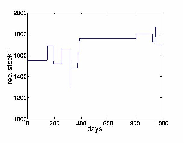
For the first stock, the Bank of Tokyo-Mitsubishi, p1(t-N) = 1550. By setting x = 0 and r = n the original price series is reconstructed exactly.
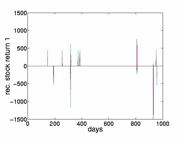
The thresholded returns of the four most dominant ICs are shown in Figure 8, and the stock price reconstructed from the thresholded return values are shown in Figure 9. The figures indicate that the thresholded ICs provide useful morphological information and can extract the turning points of original time series.
4.4 Comparison with PCAPCA is a well established tool in finance. Applications range from Arbitrage Pricing Theory and factor models to input selection for multi-currency portfolios [58]. Here we seek to compare the performance of PCA with ICA. Singular value decomposition (SVD) is used to obtain the principal components as follows. Let X denote the N ×n data matrix, where N is the number of observed vectors, and each vector has n components (usually N >> n). The data matrix can be decomposed into
where U is an N ×n column orthogonal matrix, S is an n ×n diagonal matrix consisting of the singular values and V is an n ×n matrix. The principal components are given by XV = US , ie., the vectors of the orthonormal columns in U, weighted by the singular values from S. In Figure 10 the four most dominant PCs corresponding to the Bank of Tokyo-Mitsubishi are shown. Figure 11 shows the reconstructed price obtained using the four most dominant PCs and compares it to the sum of the remaining 24 nondominant PCs. The results from the PCs obtained from the stock returns reveal the following aspects:
For the experiment reported here, the four most dominant PCs are the same, whether ordered in terms of variance or using the LĄ norm as in the ICA case. Beyond that the orders change.
Figure 13 shows the reconstructed stock price from the thresholded returns are a poor fit to the overall shape of the original price. This implies that key high level transients that were extracted by ICA are not obtained through PCA.
In summary, while PCA also decomposes the original data, the PCs do not possess the high order independence obtained of the ICs. A major difference emerges when only the largest shocks of the estimated sources are used. While the cumulative sum of the largest IC shocks retains the overall shape, this is not the case for the PCs. 5 ConclusionsThis paper applied independent component analysis to decompose the returns from a portfolio of 28 stocks into statistically independent components. The components of the instantaneous vectors of observed daily stocks are statistically dependent; stocks on average move together. In contrast, the components of the instantaneous daily vector of ICs are constructed to be statistically independent. This can be viewed as decomposing the returns into statistically independent sources. On three years of daily data from the Tokyo stock exchange, we showed that the estimated ICs fall into two categories, (i) infrequent but large shocks (responsible for the major changes in the stock prices), and (ii) frequent but rather small fluctuations (contributing only little to the overall level of the stocks). We have shown that by using a portfolio of stocks, ICA can reveal some underlying structure in the data. Interestingly, the `noise' we observe may be attributed to signals within a certain amplitude range and not to signals in a certain (usually high) frequency range. Thus, ICA gives a fresh perspective to the problem of understanding the mechanisms that influence the stock market data. In comparison to PCA, ICA is a complimentary tool which allows the underlying structure of the data to be more readily observed. There are clearly many other avenues in which ICA techniques can be applied to finance. AcknowledgementsWe are grateful to Morio Yoda, Nikko Securities, Tokyo for kindly providing the data used in this paper, and to Jean-François Cardoso for making the source code for the JADE algorithm available. Andrew Back acknowledges support of the Frontier Research Program, RIKEN and would like to thank Seungjin Choi and Zhang Liqing for helpful discussions. Andreas Weigend acknowledges support from the National Science Foundation (ECS-9309786), and would like to thank Fei Chen, Elion Chin and Juan Lin for stimulating discussions. AppendixThe experiments used the following 28 stocks:
References
Footnotes:1 We are only aware of [5] who use a neural network that maximizes output entropy and of [40,41,42,60] who apply ICA in the context of state space models for interbank foreign exchange rates to improve the separation between observational noise and the ``true price.'' 2 ICA algorithms based on second order statistics have also been proposed [7,56]. 3 For four zero-mean variables yi, yj, yk, yl, the fourth order cumulant is given by
This is the difference between the expected value E[ ·] of the product of the four variables (fourth moment), and the three products of pairs of covariances (second moments). The diagonal elements (i = j = l = m) are the fourth order self-cumulants. 4 A signal x(t) is considered to be stationary if the expected value is constant, or, after removing a constant mean, E[x(t)] = 0. In practice however, this definition depends on the interval over which we wish to measure the expectation. 5 We chose a subset of available historical data on which to test the method. This allows us to reserve subsequent data for further experimentation. 6 We also explored the effect of reducing the number of stocks that entered the ICA. The result is that the signal separation degrades when only fewer stocks are used. In that case, the independent components appear to give less distinct information. We had access to data for a maximum of 28 stocks. 7 ICs can by sorted in various ways. For example, in the implementation of the JADE algorithm Cardoso used a Euclidean norm to sort the rows of the demixing matrix W according to their contribution across all signals[14]. File translated from TEX by TTH, version 1.57. | ||||||||||||||||||||||||||||||||||||||||||||||||||||||||||||||||||||||||||||||||||||||||||||||||||||||||||||||||||||||||||||||||||||||||||||||||||||||||||||||||||||||||||||||||||||||||||||||||||||||||||||||
|
|
| Home
|
|
|
|
Copyright © 1989-2008 Andrew Back. All Rights Reserved. |